Direct collocation methods for optimal control include Euler, Runge-Kutta, Hermite-Simpson, and pseudospectral schemes. Among these, pseudospectral methods have drawn considerable attention because they combine computational efficiency and accuracy with good convergence behavior and relatively low sensitivity to initial guesses.
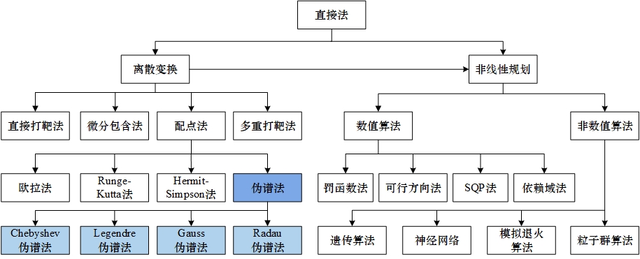
A pseudospectral method differs from ordinary collocation by using global polynomials as basis functions. The state and control are interpolated at a set of discrete nodes, and Gauss quadrature is used to enforce the differential-algebraic equations at those nodes. Four node families are common: Chebyshev-Gauss-Lobatto (CGL), Legendre-Gauss-Lobatto (LGL), Legendre-Gauss (LG), and Legendre-Gauss-Radau (LGR). These nodes are roots of Legendre polynomials or of linear combinations involving a Legendre polynomial and its derivative. CGL nodes lead to the Chebyshev pseudospectral method (CPM); LGL nodes to the Lobatto pseudospectral method (LPM), also called the Legendre pseudospectral method; LG nodes to the Gauss pseudospectral method (GPM); and LGR nodes to the Radau pseudospectral method (RPM). RPM is emphasized here because it satisfies the costate mapping theorem and generally offers better approximation accuracy and convergence speed than the other node choices.
RPM formulation
The time interval t in [t0, tf] is mapped to tau in [-1, 1) or (-1, 1] by
tau = (2t - tf - t0) / (tf - t0),
t = ((tf - t0) / 2) tau + (tf + t0) / 2.
RPM uses the zeros of P_{n-1}(tau) + P_n(tau), the n-th LGR points tau_n for n = 1, 2, ..., N, together with tau_0 = -1. The state and control are approximated by Lagrange interpolation:
X(tau) = sum_{i=0}^{N} L_i(tau) X(tau_i),
U(tau) = sum_{k=1}^{N} Ltilde_k(tau) U(tau_k).
Notice the different starting indices: the state expansion includes the initial node i = 0, while the control expansion starts at k = 1. Here P_n is the Legendre polynomial, and the Lagrange basis satisfies L_i(tau_j) = 1 when i = j and 0 otherwise. The interpolation error decreases faster as N increases.
Differentiating the approximate state gives
Xdot(tau_k) = sum_{i=0}^{N} DotL_i(tau_k) X(tau_i) = sum_{i=0}^{N} D_{ki} X(tau_i),
where D_{ki} is the differential matrix. The differential equation constraint then becomes the algebraic condition
F_k = sum_{i=0}^{N} D_{ki} X(tau_i) - ((tf - t0) / 2) f(X(tau_k), U(tau_k)) = 0,
for k = 1, 2, ..., N.
The objective is discretized with Gauss quadrature:
J ≈ Phi(x(t0), t0, x(tf), tf) + ((tf - t0) / 2) sum_{k=1}^{N} w_k g(X(tau_k), U(tau_k), tau_k; t0, tf),
where the weights w_k are obtained by integrating the Lagrange basis over [-1, 1]. The continuous optimal control problem is therefore converted into a nonlinear programming problem. The design variables are the states (X_0, X_1, ..., X_N), the controls (U_1, U_2, ..., U_N), and the initial and final times t0 and tf. The constraints consist of the differential equation conditions (F_1, ..., F_N) = 0, the boundary condition phi(X(tau_0), X(tau_N)) = 0, and the path constraints C(X(tau_k), U(tau_k), tau_k; t0, tf) ≤ 0 for k = 1, 2, ..., N.
How the pseudospectral variants compare
The costate mapping principle asks whether the Karush-Kuhn-Tucker conditions of the nonlinear programming problem are consistent with the discretized first-order necessary conditions of the original continuous optimal control problem. If they are, the costates of the continuous problem can be estimated from the Lagrange multipliers of the NLP, which means the NLP solution can be interpreted as the solution of the original optimal control problem.
In terms of approximation accuracy, GPM and RPM are better than LPM for states, controls, and costates. All three converge exponentially, but GPM and RPM converge faster than LPM. For problems of the same size, the computation times of LPM, GPM, and RPM are not dramatically different. GPM and RPM satisfy the costate mapping principle, whereas LPM does not. RPM has one additional practical advantage: the control at the initial point can be recovered directly from the NLP solution, while GPM cannot do this. In hp-pseudospectral implementations, this property allows RPM to omit the continuity equations between segments, reducing the number of constraints and simplifying the implementation compared with GPM.
Node distribution and the Runge phenomenon
Node placement is a key distinction among collocation schemes. Ordinary collocation often divides the time interval uniformly, but uniform nodes can produce the Runge phenomenon, as shown below.
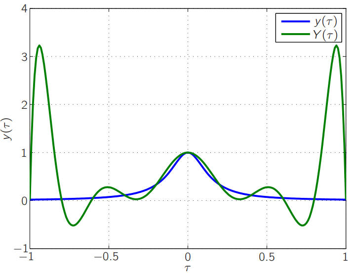
For y(tau) = 1 / (1 + 50 tau^2) on [-1, 1], a high-order interpolant Y(tau) can oscillate strongly near the ends of the interval, causing large errors at the edges. Pseudospectral methods avoid this by mapping t in [t0, tf] to tau in [-1, 1] and using nonuniform nodes such as LG, LGR, and LGL points.
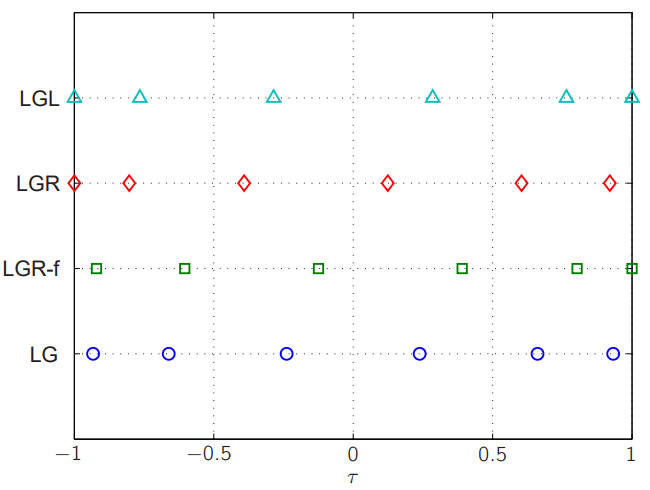
LG nodes are the zeros of the Legendre polynomial P_n(tau). LGR nodes are the zeros of P_{n-1}(tau) + P_n(tau). LGL nodes are the stationary points of P_{n-1}(tau), that is, the points where its derivative vanishes. Legendre nodes are sparse in the middle and denser near the boundaries. LG nodes do not include either endpoint tau = -1 or tau = 1. LGR nodes include one endpoint, either tau = -1 or tau = 1. LGL nodes include both endpoints. The distribution for six nodes is illustrated below.
Why LGL and CGL do not satisfy costate mapping
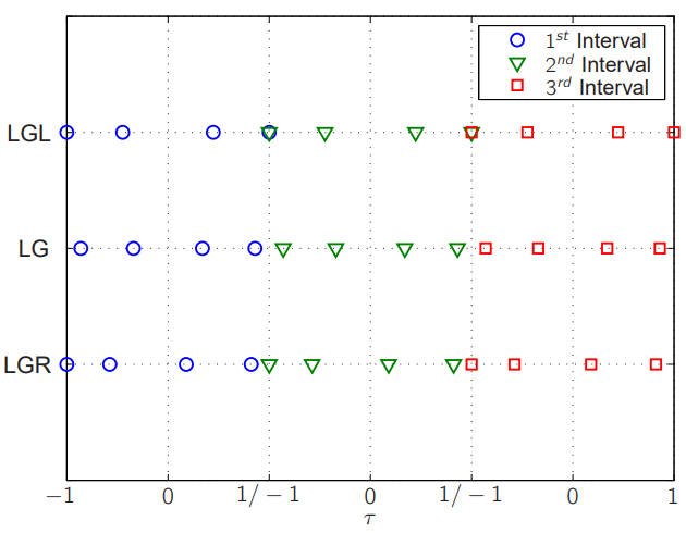
LGL nodes include both boundary points tau = -1 and tau = 1. At those boundary points, the discrete form of the dynamics is not satisfied in the same way, so the costate variables cannot be estimated accurately. As a result, the optimal control problem cannot be transformed equivalently into the NLP problem.
The issue is a coupling effect at the shared endpoint between adjacent intervals. Garg notes that at the boundary points, the discrete equivalents of the continuous boundary conditions are coupled in the discrete costate dynamics. Because neighboring intervals share an endpoint but use different formulas, the costate estimate at that point is inaccurate, and the costate mapping theorem fails. LGR and LG nodes do not occupy both endpoints within an interval, so this coupling does not occur, and the costate mapping theorem holds. CGL nodes also include both endpoints, so CGL likewise fails to satisfy costate mapping.
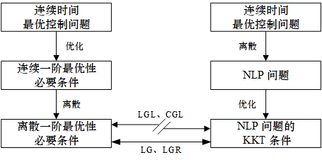
Solution procedure
The practical workflow is straightforward. First, choose the number of discretization points, the time span, the number of subintervals, and initial guesses for the state and control. Second, compute the nodes for the chosen collocation scheme. Third, write the constraint equations correctly; this step is critical to whether the pseudospectral method succeeds. Fourth, discretize the objective function. Finally, solve the resulting NLP, for example with MATLAB's fmincon.
Example problem
Consider the system
xdot = -x^2 + u, x0 = 10,
with the performance index
J(u) = 0.5 ∫_0^1 (x^2 + u^2) dt.
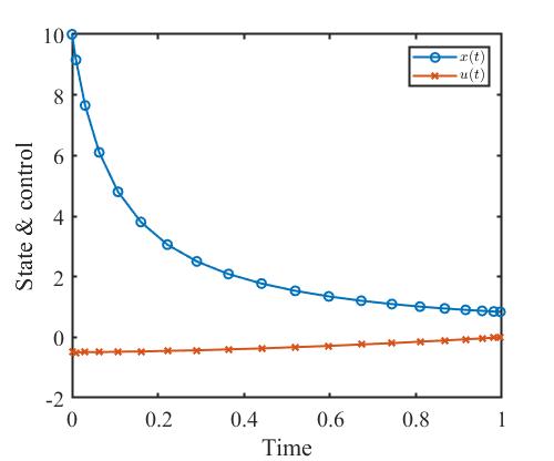
The goal is to find the optimal control that minimizes J. This example is taken from Optimization and Optimal Control, 2nd ed., p. 257, Example 13.1.
The following MATLAB code implements the pseudospectral solution and includes LGR, LGL, and CGL node options.
%--------------------------------------------------------------------------
% Method_Pseudospectral.m
% Attempt to solve the Bryson-Denham problem using a pseudospectral method
% (namely LGL nodes and Gaussian quadrature)
%--------------------------------------------------------------------------
%
%--------------------------------------------------------------------------
% Primary Contributor: Daniel R. Herber, Graduate Student, University of
% Illinois at Urbana-Champaign
% https://github.com/danielrherber/optimal-control-direct-method-examples
%--------------------------------------------------------------------------
%--------------------------------------------------------------------------
% Description: Solve an unconstrained optimal control problem using a pseudospectral method
% Example: Optimization and Optimal Control, 2nd ed., p. 257, Example 13.1
% Type: optimal control problem without control constraints
% Date: 2022/07/07
%--------------------------------------------------------------------------
clear;clc;close all;

%% 01 Initial parameter settings
p.ns = 1; p.nu = 1;                     % number of state and control variables
p.t0 = 0; p.tf = 1;                     % initial and final time
p.x0 = 10;                              % initial condition

p.nt = 20;                              % number of collocation points
% p.method = 'LGL';                       % choose collocation scheme: Legendre-Gauss-Lobatto (LGL)
% p.method = 'CGL';                       % or Chebyshev-Gauss-Lobatto (CGL)
p.method = 'LGR';                       % or Legendre-Gauss-Radau (LGR)
if strcmp(p.method,'LGL')
    p.tau = LGL_nodes(p.nt-1);          % discretize time interval into [-1,1]
    p.D   = LGL_Dmatrix(p.tau);         % differentiation matrix
    p.w   = LGL_weights(p.tau);         % collocation weights
elseif strcmp(p.method,'CGL')
    p.tau = CGL_nodes(p.nt-1);          % discretize time interval into [-1,1]
    p.D   = CGL_Dmatrix(p.tau);         % differentiation matrix
    p.w   = CGL_weights(p.tau);         % collocation weights
elseif strcmp(p.method,'LGR')
    [p.tau,p.w] = LGR_nodes_and_weights(p.nt-1);
    p.D   = LGR_Dmatrix(p.tau);         % differentiation matrix
end

% collect variables as x = [x,u]
p.x_index = 1:p.nt;
p.u_index = p.nt+1:2*p.nt;

%% 02 Solution algorithm
% initial guess for [x;u]
y0 = zeros(p.nt*(p.ns+p.nu),1);
% solver settings
options = optimoptions(@fmincon,'display','iter','MaxFunEvals',1e5,'algorithm','sqp');

tic;
[y,fval] = fmincon(@(y) objective(y,p),y0,[],[],[],[],[],[],@(y) constraints(y,p),options);
toc;

% extract solution
p.x = y(p.x_index);                     % state
p.u = y(p.u_index);                     % control
p.t = tau2t(p);                         % transform time variable from tau to t

%% 03 plotting
window_width = 500;
window_height = 416;

% state
k = 1;
figure('color',[1 1 1],'position',[300+k*window_width,300,window_width,window_height]);
plot(p.t, p.x, 'o-', 'LineWidth',1.5);hold on;
plot(p.t, p.u, 'x-', 'LineWidth',1.5);
xlabel('Time');
ylabel('State & control');
set(gca,'FontSize',15,...
        'FontName','Times New Roman',...
        'LineWidth',1.5);
legend('$x(t)$','$u(t)$',...
        'Location','Northeast',...
        'FontSize',10,...
        'interpreter','latex');

% save data
% .\ next-level folder
% ..\ parent folder
% save(['..\','pseudospectral_method.mat']);
%% 04 Subfunctions
% objective function
function J = objective(y,p)
    % get state and control
    x = y(p.x_index);
    u = y(p.u_index);

    L = u.^2 + x.^2;                    % integrand
    J = (p.tf-p.t0)/2 * dot(p.w,L)/2;   % compute objective
end

% constraint function
function [c,ceq] = constraints(y,p)
    % get state and control
    x = y(p.x_index);
    u = y(p.u_index);
    % state equation constraints
    Y = x; F = (p.tf-p.t0)/2*(-x.^2+u);
    % initial state constraint
    ceq1 = x(1) - p.x0;
    ceq2 = p.D*Y - F;
    % output constraints
    ceq = [ceq1;ceq2(:)];
    c = [];
end

% transform tau to t
function t = tau2t(p)
    % following Eq. (4.25) on p. 79 of Space-Based Earth-Strike Weapon Orbit Planning and Guidance Technology (2013)
    t = (p.tf-p.t0)*p.tau/2+(p.tf-p.t0)/2;
end
The resulting state and control histories are shown below.
Timing comparison
The computational times of RPM, LPM, CPM, single shooting, and multiple shooting were compared at 20, 30, 40, and 50 discretization points. The laptop used for the test was a Lenovo ThinkPad T490 with an Intel Core i5-8265U CPU at 1.60 GHz, 8 GB DDR4 2400 MHz plus 8 GB DDR4 2667 MHz memory, and the balanced power mode.
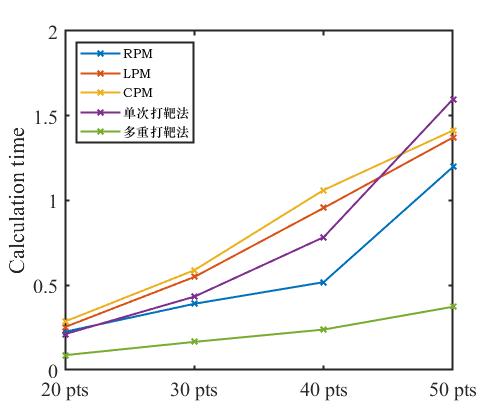
The table gives the timing values directly.
<table> <thead> <tr> <th></th> <th>RPM</th> <th>LPM</th> <th>CPM</th> <th>Single shooting</th> <th>Multiple shooting</th> </tr> </thead> <tbody> <tr> <td>20 points</td> <td>0.2255</td> <td>0.2535</td> <td>0.2861</td> <td>0.2116</td> <td>0.0875</td> </tr> <tr> <td>30 points</td> <td>0.3905</td> <td>0.5488</td> <td>0.5888</td> <td>0.4328</td> <td>0.1659</td> </tr> <tr> <td>40 points</td> <td>0.5183</td> <td>0.9558</td> <td>1.0617</td> <td>0.7834</td> <td>0.2385</td> </tr> <tr> <td>50 points</td> <td>1.1985</td> <td>1.3719</td> <td>1.4135</td> <td>1.5981</td> <td>0.3731</td> </tr> </tbody> </table>Multiple shooting is the fastest in this comparison, followed by RPM, then single shooting, with LPM and CPM taking longer. The timing table makes the practical trade-off clear: multiple shooting is fastest here, while RPM offers a strong balance of accuracy, convergence behavior, and costate mapping.